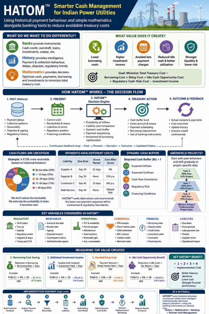
HATOM™: Smarter Cash Management for Indian Power Utilities

HATOM™ — Historical Adaptive Treasury Optimization Model

Using historical payment behaviour and simple mathematics alongside banking tools to reduce avoidable treasury costs

What should be done differently?

Indian electricity utilities already have a wide range of banking instruments for managing liquidity. They use cash-credit facilities, overdrafts, working-capital loans, sweep accounts, fixed deposits, short-term investments and other treasury arrangements.

Our proposition is not to replace these banking tools.

It is to change the decision-making process that determines when, how much and for how long those instruments should be used.

Today, many treasury decisions are still substantially dependent on management experience and conventional cash-flow forecasting. A utility may maintain a large cash balance because it is uncertain when receivables will arrive, while simultaneously using short-term borrowing facilities to manage periodic liquidity requirements.

Our proposition is simple:

Use the utility’s own historical cash-flow behaviour to quantify uncertainty, combine it with current regulatory and contractual information, and use simple mathematical optimization to determine the most economical treasury action.

The objective is not merely to predict cash.

The objective is to reduce the total cost of managing cash.

We call this approach the Historical Adaptive Treasury Optimization Model — HATOM™.

Its philosophy can be summarized in one sentence:

Banks provide the instruments. History provides the intelligence. Mathematics provides the decision.

1. Why cash management is different in the electricity sector

Cash management in the electricity sector is structurally different from that of many conventional businesses.

Electricity utilities operate within a framework involving:

• • regulated tariffs;

• • long-term PPAs;

• • government-owned or financially constrained counterparties;

• • subsidy mechanisms;

• • regulatory approvals;

• • fuel and transportation arrangements;

• • statutory payment obligations;

• • debt servicing requirements;

• • electricity-market transactions.

Consequently, the utility may have substantial receivables but still experience liquidity stress.

A generating company may have ₹1,000 crore of legitimate receivables but receive only a portion on the contractual due dates.

A DISCOM may have billed its customers but await subsidy reimbursement.

A transmission utility may have predictable contractual revenues but face temporary mismatches between collections and its own payment obligations.

The fundamental problem is therefore often not whether the money will eventually be received, but when the money will actually be available.

At the same time, many outgoing payments cannot simply be postponed indefinitely.

The utility must make payments towards:

• • coal and fuel;

• • railways;

• • transmission charges;

• • debt servicing;

• • salaries;

• • statutory dues;

• • EPC contracts;

• • O&M expenses;

• • other suppliers.

Treasury therefore operates in an environment where:

Cash inflows may be uncertain in timing, while cash outflows may be fixed by contract, regulation or operational necessity.

This creates a classic timing mismatch problem.

2. The underutilized asset: historical cash-flow behaviour

Electricity utilities possess something extremely valuable—years of actual transaction data.

Most utilities can identify:

• • invoice dates;

• • contractual due dates;

• • actual receipt dates;

• • payment delays;

• • ageing;

• • disputed amounts;

• • subsidy receipts;

• • tariff adjustments;

• • supplier payment patterns;

• • borrowing requirements;

• • investment balances;

• • interest costs.

Yet historical information is often used primarily for accounting, reporting and audit rather than as an active input into daily treasury decision-making.

This represents a significant opportunity.

Suppose a particular DISCOM has historically paid a generating company:

• • 20% of invoices within the contractual period;

• • 40% within the following 15 days;

• • 25% within 30 days;

• • 10% within 60 days;

• • 5% after 60 days.

The important information is not that the utility has a ₹100 crore receivable.

The important information is the probability distribution of when that ₹100 crore is likely to become cash.

The ₹100 crore remains ₹100 crore.

HATOM™ does not reduce the receivable because it is delayed.

Instead, it estimates the probability that different amounts will become available at different points in time.

That distinction is central to the model.

3. From cash forecasting to cash optimization

Traditional treasury forecasting may say:

“₹400 crore is expected to be received during the month.”

HATOM™ asks a more useful question:

“How much of the ₹400 crore is likely to be available on each relevant date, given historical payment behaviour and current circumstances?”

This allows treasury to construct a probabilistic cash-flow profile.

For example:

The model can then combine this information with upcoming liabilities.

The objective is no longer simply to forecast the closing bank balance.

It becomes:

What level of liquidity should be maintained, and what should be done with the remaining cash?

4. The liability side is equally important

The same logic must be applied to payments.

A liability of ₹100 crore remains a ₹100 crore liability.

The model does not assume that a ₹100 crore payment can be arbitrarily reduced to ₹80 crore because of cash constraints.

Instead, HATOM™ evaluates timing.

Consider a supplier payment of ₹100 crore:

• • contractual due date: Day 30;

• • contractual grace period: up to Day 45;

• • late-payment interest after Day 45: 12% per annum.

If the utility faces a temporary liquidity shortage on Day 30, several alternatives may exist:

1. 1. Borrow ₹100 crore and pay immediately.

1. 1. Use available cash and postpone another flexible payment.

1. 1. Use the contractual grace period and pay on Day 40.

1. 1. Deploy temporary surplus cash elsewhere and settle the liability later, if contractually permissible.

The model compares the economic cost of these alternatives.

The decision is therefore not:

“Can we delay payment?”

It is:

“What is the economically optimal timing of this payment, subject to the contractual, regulatory and operational constraints?”

5. The HATOM™ mathematical objective

At its simplest level, HATOM™ seeks to minimize the total economic cost of treasury management.

The objective can be expressed as:

Minimize Total Treasury Cost = Borrowing Cost + Delay Cost + Idle-Cash Opportunity Cost + Regulatory Cash-Risk Cost − Investment Income

The four principal costs are:

Borrowing Cost

Interest paid on:

• • working-capital loans;

• • cash-credit facilities;

• • overdrafts;

• • short-term borrowings;

• • other liquidity facilities.

Delay Cost

Costs associated with delaying payments, including:

• • late-payment surcharge;

• • contractual interest;

• • penalties;

• • other financial consequences.

Idle-Cash Opportunity Cost

The economic value foregone when unnecessarily large cash balances are maintained instead of being:

• • invested;

• • used to reduce borrowing;

• • deployed elsewhere within treasury policy.

Regulatory Cash-Risk Cost

The expected financial effect of uncertain cash inflows associated with:

• • tariff proceedings;

• • truing-up;

• • disputed receivables;

• • regulatory assets;

• • subsidy reimbursement;

• • appellate proceedings;

• • litigation;

• • delayed implementation of regulatory orders.

Against these costs, the model considers:

Investment Income

Returns generated by appropriately deploying temporary surplus cash through permitted banking and investment instruments.

The model therefore does not seek to minimize borrowing alone.

It seeks to minimize the total economic cost of liquidity management.

6. Why this can create financial value

Consider a simplified example.

A utility has:

Cash available: ₹500 crore

Payments expected over the next 30 days: ₹350 crore

Expected receipts: ₹400 crore

Conventional treasury practice may retain a substantial cash balance because the timing of receipts is uncertain.

But historical data may demonstrate that most of the expected receipts are highly likely to arrive before the critical payment dates.

Suppose HATOM™ determines that the utility needs only ₹300 crore as a risk-adjusted liquidity buffer.

The remaining ₹200 crore may potentially be:

• • invested;

• • used to reduce expensive short-term borrowing;

• • placed in an appropriate sweep arrangement;

• • or otherwise deployed according to treasury policy.

If this decision is repeated across the year, even a relatively small percentage improvement in treasury efficiency can create substantial financial value.

The model does not have to predict every receipt perfectly.

It only needs to make better decisions than the existing process on a sufficiently consistent basis.

7. Dynamic Cash Buffer

One of the most practical outputs of HATOM™ is a dynamic cash buffer.

Traditional practice may establish:

“Maintain ₹300 crore minimum cash.”

HATOM™ asks:

“What minimum cash balance is appropriate today, given expected inflows, expected outflows, cash-flow uncertainty, regulatory risk and financing conditions?”

The required cash buffer can be expressed conceptually as:

Required Cash Buffer = f(Expected Inflows, Expected Outflows, Cash-flow Uncertainty, Regulatory Risk, Financing Conditions)

The buffer therefore depends on:

• • expected cash inflows;

• • expected cash outflows;

• • historical variability;

• • regulatory and commercial risk;

• • cost and availability of alternative financing.

The result is a dynamic rather than fixed liquidity reserve.

A period with high regulatory uncertainty may justify a larger buffer.

A period with highly predictable collections may justify a lower buffer.

This creates an important opportunity for utilities to reduce unnecessary idle cash without compromising liquidity.

8. Regulatory uncertainty must be quantified

Electricity-sector cash management cannot be properly optimized without considering regulatory uncertainty.

A ₹500 crore receivable that has already been admitted by the regulator and is awaiting payment is economically different from a ₹500 crore receivable that is subject to substantial dispute and litigation.

Similarly, a subsidy receivable backed by an established government mechanism is different from an amount that depends upon a future administrative decision.

HATOM™ therefore proposes classifying receivables according to their degree of certainty.

For example:

Category A – High Certainty

• • admitted amount;

• • undisputed;

• • no material stay;

• • normal payment history.

Category B – Moderate Certainty

• • payment historically delayed;

• • subsidy dependent;

• • implementation pending.

Category C – High Uncertainty

• • disputed;

• • under appeal;

• • subject to stay;

• • dependent on unresolved regulatory or judicial proceedings.

The model can assign different probability distributions to each category.

The objective is not to predict the outcome of litigation.

The objective is to avoid treating uncertain receivables as though they were equivalent to cash in the bank.

9. The six intelligence layers of HATOM™

HATOM™ integrates six categories of information.

These layers feed a common treasury decision engine.

The output is not merely another report.

It is a set of recommended treasury actions.

10. Payment sequencing as an optimization problem

Not every payment has the same economic consequence when delayed.

Consider:

If cash is temporarily constrained, the treasury department should not necessarily treat all four payments identically.

The model can rank payment alternatives according to:

• • contractual cost;

• • financial cost;

• • operational consequence;

• • regulatory consequence;

• • supplier relationship;

• • availability of alternative liquidity.

This produces an economically optimized payment sequence.

Importantly, HATOM™ is not a recommendation to routinely delay payments.

It is a framework for identifying the least-cost and lowest-risk timing of payments within permissible contractual and regulatory boundaries.

11. Banking instruments remain essential

HATOM™ is not intended to replace existing banking arrangements.

It is an intelligence layer above them.

Suppose the model determines:

“₹150 crore of surplus cash is likely to remain available for approximately 12 days.”

Treasury can then decide whether the appropriate instrument is:

• • a sweep arrangement;

• • short-term deposit;

• • overnight deployment;

• • liquid investment;

• • repayment of a high-cost borrowing facility.

Similarly, if HATOM™ identifies a probable temporary deficit, treasury can compare:

• • overdraft;

• • cash-credit drawdown;

• • short-term borrowing;

• • liquidation of an investment;

• • acceleration of a collection;

• • payment sequencing.

Thus:

HATOM™ decides the economics; the banking system executes the decision.

12. Greenfield projects: what happens when there is no history?

HATOM™ is not restricted to operating assets.

It can also be applied to:

• • new thermal generating stations;

• • solar projects;

• • wind projects;

• • pumped storage projects;

• • transmission projects;

• • new distribution businesses.

The obvious problem is that a greenfield project has no historical payment behaviour.

The solution is to begin with comparable-project behaviour.

For example, a new generating project may initially use information from:

• • similar projects;

• • the same counterparty;

• • comparable PPAs;

• • similar regulatory structures;

• • comparable financing arrangements;

• • historical commissioning experience.

The behavioural estimate can be represented simply as:

Current Behaviour Estimate = (Peer Weight × Peer Behaviour) + (Project Weight × Project Behaviour)

with:

Peer Weight + Project Weight = 100%

At project commencement, peer information dominates.

As the project accumulates actual experience, the model gradually shifts towards project-specific information.

For example:

Year 0: 90% peer information + 10% project information

Year 1: 60% peer information + 40% project information

Year 2: 30% peer information + 70% project information

Mature project: predominantly project-specific information.

The weights can be determined according to the quantity and quality of available data.

This allows HATOM™ to operate throughout the project life cycle.

13. The variables that matter

A sector-specific model must recognize that electricity-sector cash flows are influenced by many variables.

Regulatory variables

• • tariff order pending;

• • provisional tariff;

• • final tariff;

• • truing-up;

• • carrying-cost recovery;

• • fuel-cost adjustment;

• • regulatory asset recovery;

• • subsidy reimbursement;

• • APTEL proceedings;

• • Supreme Court proceedings;

• • regulatory stays.

Receivable variables

• • invoice amount;

• • due date;

• • actual receipt date;

• • ageing;

• • disputed amount;

• • admitted amount;

• • amount under appeal;

• • counterparty payment history.

Operational variables

• • PLF;

• • plant availability;

• • forced outages;

• • planned maintenance;

• • auxiliary consumption;

• • renewable generation;

• • coal inventory.

Commercial variables

• • PPA receipts;

• • power-exchange revenue;

• • merchant sales;

• • DSM settlement;

• • REC revenue;

• • carbon-credit revenue.

Financial variables

• • working-capital interest rate;

• • overdraft rate;

• • cash-credit limit;

• • investment yield;

• • short-term deposit rate;

• • available credit limits;

• • covenant restrictions.

Liability variables

• • contractual due date;

• • grace period;

• • late-payment surcharge;

• • supplier-specific terms;

• • operational consequences of delay.

The model does not necessarily require all these variables in its first implementation.

The principle is to start with the variables that have the greatest financial impact.

14. What data is actually required?

A sophisticated data platform is not necessary for the first implementation.

A utility can begin with approximately three to five years of historical information.

Receivables

• • invoice date;

• • due date;

• • receipt date;

• • amount;

• • counterparty;

• • dispute status;

• • regulatory status.

Payables

• • invoice date;

• • contractual due date;

• • actual payment date;

• • grace period;

• • applicable interest;

• • supplier.

Treasury

• • opening cash;

• • closing cash;

• • borrowing;

• • repayment;

• • borrowing interest;

• • investments;

• • investment income.

Regulatory

• • pending tariff proceedings;

• • true-up;

• • subsidy status;

• • litigation;

• • regulatory assets;

• • material regulatory adjustments.

Much of this information already exists within ERP, billing, finance and regulatory systems.

The initial challenge is therefore not necessarily the creation of new data.

It is bringing existing information together for decision-making.

15. The model can begin in Excel

One of the strengths of HATOM™ is that its initial implementation does not require artificial intelligence.

The first version can use:

• • historical averages;

• • median payment delays;

• • standard deviation;

• • payment-delay distributions;

• • simple probability scores;

• • scenario analysis;

• • cash-flow matching;

• • Excel Solver.

This allows a utility to test the proposition at relatively low cost.

If measurable savings are demonstrated, the methodology can subsequently evolve into:

• • stochastic optimization;

• • Monte Carlo simulation;

• • Bayesian updating;

• • machine learning;

• • real-time ERP integration;

• • AI-assisted treasury management.

The sophistication of the mathematics can therefore grow after the economic value has been demonstrated, rather than before.

16. Measuring the value created

HATOM™ should ultimately be judged by financial outcomes, not mathematical sophistication.

Reduction in borrowing cost

Borrowing Cost Saving = Reduction in Borrowing × Borrowing Rate × Days / 365

For example, if ₹100 crore of borrowing is avoided for 30 days at an annual borrowing rate of 9%:

Saving = ₹100 crore × 9% × 30 / 365

This produces approximately ₹0.74 crore, or ₹7.4 lakh, of interest saving.

Additional investment income

Investment Income = Surplus Cash Invested × Investment Yield × Days / 365

If ₹100 crore is invested for 30 days at 6%:

Income = ₹100 crore × 6% × 30 / 365

This produces approximately ₹0.49 crore, or ₹4.9 lakh, of additional income.

Avoided delay cost

Avoided Delay Cost = Payment Amount × Applicable Delay Interest Rate × Days / 365

For example, a ₹100 crore payment carrying a 12% annual delay charge for 20 days represents:

Cost = ₹100 crore × 12% × 20 / 365

or approximately ₹0.66 crore.

The model can compare this cost against the alternative cost of borrowing or deploying available cash.

Reduction in idle-cash opportunity cost

Opportunity Benefit = Reduction in Idle Cash × Relevant Alternative Return × Days / 365

Thus, if ₹100 crore that would otherwise remain idle can be economically deployed for 30 days at 6%:

Benefit = ₹100 crore × 6% × 30 / 365

This represents approximately ₹0.49 crore of additional economic value.

Overall benefit

The aggregate value can therefore be represented as:

Net HATOM Benefit = Borrowing Cost Saving + Investment Income + Avoided Delay Cost + Idle-Cash Opportunity Benefit − HATOM Implementation Cost

This gives management a straightforward measure of whether the framework is producing value.

17. From descriptive treasury to prescriptive treasury

There is a fundamental difference between conventional treasury reporting and HATOM™.

Conventional treasury reporting

Receivables: ₹2,000 crore
Cash: ₹400 crore
Borrowing: ₹150 crore
Payments due: ₹350 crore

This tells management what has happened or what is currently scheduled.

HATOM™ approach

Based on historical realization behaviour, current regulatory status and upcoming liabilities, the probability of a liquidity deficit during the next 30 days is estimated at X%. The recommended minimum cash buffer is ₹Y crore. ₹Z crore may be deployed for approximately N days. Liability A should be settled immediately, while Liability B can economically be settled later within its contractual grace period. Borrowing should be drawn only when the projected liquidity position requires it.

The first is descriptive.

The second is prescriptive.

That is the central change proposed by HATOM™.

18. A practical implementation roadmap

A utility does not need to transform its entire treasury operation immediately.

A pilot can begin with one business unit or one major cash-flow stream.

Step 1 — Build the historical database

Collect three to five years of receivable, payable and treasury data.

Step 2 — Analyse payment behaviour

Determine:

• • average delay;

• • median delay;

• • variability;

• • counterparty-specific behaviour;

• • seasonal patterns.

Step 3 — Classify receivables

Separate:

• • highly certain;

• • moderately uncertain;

• • disputed;

• • regulatory;

• • litigation-related receivables.

Step 4 — Map liabilities

For each major liability identify:

• • due date;

• • grace period;

• • interest;

• • penalty;

• • operational consequences.

Step 5 — Build a rolling cash model

Initially use:

• • 30-day;

• • 60-day;

• • 90-day horizons.

Step 6 — Introduce the dynamic cash buffer

Calculate the liquidity reserve required under different scenarios.

Step 7 — Optimize deployment and borrowing

Compare:

• • idle cash;

• • investment;

• • borrowing;

• • payment timing.

Step 8 — Measure actual results

Compare the model’s recommendation against actual treasury decisions.

The objective is to establish measurable:

• • interest savings;

• • investment income;

• • reduction in idle cash;

• • reduction in unnecessary borrowing.

Once demonstrated, the model can be expanded.

19. The HATOM™ architecture

The complete framework can be viewed as a continuous decision cycle.

PAST

Historical cash-flow data
↓
Payment and collection behaviour
↓

PRESENT

Current cash

• • Current receivables

• • Current liabilities

• • Regulatory status

• • Financing conditions
    ↓

HATOM™ DECISION ENGINE

↓

TREASURY ACTION

• • Dynamic cash buffer

• • Investment amount

• • Investment tenure

• • Payment sequencing

• • Borrowing requirement

• • Scenario-based liquidity requirement

↓

ACTUAL OUTCOME

↓

The actual outcome becomes new historical data.

This creates a continuous feedback loop:

Past → Present → Decision → Outcome → Updated History

This is the adaptive element of HATOM™.

20. Why this approach is particularly relevant now

The financial environment of the electricity sector is becoming increasingly complex.

Utilities must simultaneously manage:

• • growing renewable integration;

• • changing power-market structures;

• • large capital expenditure;

• • working-capital requirements;

• • regulatory adjustments;

• • delayed receivables;

• • financing costs;

• • increasingly sophisticated banking arrangements.

At the same time, utilities are generating enormous quantities of financial and operational data.

The opportunity is therefore not necessarily to create another financial instrument.

It is to make better use of the information already available.

Even a modest improvement in treasury efficiency, when applied to a utility handling thousands of crores of annual cash flows, can create meaningful recurring value.

21. Conclusion: From banking-led to intelligence-led treasury

Indian electricity utilities do not necessarily need another banking instrument.

They need to extract more value from the instruments they already possess.

The opportunity lies in connecting:

Historical cash-flow behaviour

with

Regulatory and commercial intelligence

and

mathematical decision-making.

HATOM™ proposes a practical transition from:

Banking-led cash management

to

Data-informed, mathematically optimized treasury management.

It does not require a utility to abandon managerial judgement.

It does not require sophisticated artificial intelligence from Day One.

It does not assume that receivables can be reduced simply because they are delayed.

And it does not advocate indiscriminate postponement of payments.

Instead, it asks a series of disciplined questions:

How much cash is actually required?

When is it required?

How certain are the expected receipts?

What does history tell us about the timing of those receipts?

Which payments have flexibility?

What is the economic cost of delaying them?

What is the cost of borrowing?

What return can be earned on temporary surplus cash?

What additional liquidity buffer is justified by regulatory uncertainty?

The answers can then be converted into a mathematically informed treasury decision.

The philosophy is deliberately simple:

Banks provide the instruments.

History provides the intelligence.

Mathematical Reasoning provides the decision.

HATOM™ is therefore proposed not as a final mathematical solution, but as a practical starting framework.

A utility can begin with historical data, basic statistics and an Excel model. If the resulting decisions demonstrate measurable financial benefits, the framework can progressively evolve into stochastic optimization, advanced analytics, machine learning and AI-enabled treasury management.

The mathematics can become more sophisticated over time.

The opportunity to start using the mathematics exists today.

About the Framework

HATOM™ — Historical Adaptive Treasury Optimization Model is a conceptual treasury decision-support framework proposed for the Indian electricity sector. It is designed to complement existing banking and treasury practices by incorporating historical cash-flow behaviour, regulatory uncertainty, contractual payment conditions and mathematical optimization into liquidity decisions.

Proposed by: Nomosfinergy LLP

This article presents a conceptual methodology for discussion and professional exploration. Actual implementation should consider the specific contractual, regulatory, financial, accounting, tax and treasury policies applicable to each utility. The framework does not constitute financial, investment, legal or regulatory advice.